Predicting purchases with Market Basket Analysis
Create your own “Customers who bought this also bought” section using MBA with Association Rules

Do you ever make impulse purchases? Sure you do. But, do you ever wonder why these products are so conveniently available to you even when you weren’t looking for them? All of us know about the Customers who bought this also bought section on Amazon, and the aforementioned impulse purchases happen there quite a lot.
Even in physical grocery stores, you’d find items which are complementary (e.g. Bread and Butter) on the same shelf or at least in close proximity to each other. This data of complementary items also helps the stores in giving offers and discounts on these items in some way that they deem profitable. The advertisements for one item can be targeted on customers of the other. Also, sometimes the company might come up with a combined product for the two which might increase sale.
Now, the question arises, how to find these complementary items? The answer is Market Basket Analysis.
What is Market Basket Analysis?
Market Basket Analysis (MBA) is a modelling technique based upon the theory that if you buy a certain group of items, you are more (or less) likely to buy another group of items.
For example: while at McDonald’s, if you buy sandwiches and cookies, you are more likely to buy a drink than someone who did not buy a sandwich.
In the retail industry, MBA refers to an unsupervised data mining technique that discovers co-occurrence relationships among customers’ purchase activities. The volume of sales made from user clicks on Amazon’s “Customers who bought this product also bought these products…” call to action links is a testament to the effect and importance of market basket analysis.
The objective of Market Basket Anaysis and this article is to predict with the use of previous data as to what product does a person buy after purchasing some product, or rather put simply, what relates to the previously bought product.
Some Terminologies
Now, we need to get familiar with the terminologies used here to get a clearer understanding of the topic.
Items
Items are the objects that we are identifying associations between. For an online retailer, each item is a product in the shop. For a publisher, each item might be an article, a blog post, a video etc. A group of items is an item set.
Item set, I = {i₁,i₂,i₃, … ,iₙ}Transactions
Transactions are instances of groups of items co-occurring together. For an online retailer, a transaction is, generally, a, transaction. For a publisher, a transaction might be the group of articles read in a single visit to the website. (It is up to the analyst to define over what period to measure a transaction.) For each transaction, then, we have an item set.
Transaction, tₙ = {iᵢ,iⱼ, … ,iₖ}Rules
Rules are statements of the form
{i₁,i₂, … } ⇒ {iₖ}i.e. if you have the items in item set on the left hand side (LHS) of the rule i.e. {i₁,i₂, … }, then it is likely that a visitor will be interested in the item on the right hand side (RHS i.e. {iₖ}.
For example, the sandwiches and cookies from above example become the LHS and the drink becomes the RHS.
Methodology
Association Rule Mining
- For finding frequent patterns, associations, correlations, or causal structures among sets of items in transaction databases.
- To understand customer buying habits by finding associations and correlations between the different items that customers place in their “shopping basket”.
- Rule Form:
Antecedent Item ⇒ Consequent Item
Apriori Principle
The apriori principle can reduce the number of itemsets we need to examine.
Put simply, the apriori principle states that: if an itemset is infrequent, then all its supersets must also be infrequent.
This means if {beer} was found to be infrequent, we can expect {beer, pizza} to be equally or even more infrequent. So in consolidating the list of popular item sets, we need not consider {beer, pizza}, nor any other item set configuration that contains beer.

Now, we use three very important concepts of Support, Confidence & Lift in order to implement and understand Market Basket Analysis.
Support
The support of an item or item set is the fraction of transactions in the data set that contain that item or item set. Support determines how often a rule is applicable to a given data set.
Support(A ∪ B) = min(Support(A), Support(B))Confidence
Confidence is defined as the conditional probability that a transaction containing the LHS (the antecedent item A) will also contain the RHS (the consequent item B).
Confidence(A => B) = P(B|A) = P(A ∩ B)/P(A)Confidence(A => B) = Support(A ∪ B)/Support(A)
A rule’s confidence is a measurement of its predictive power or accuracy. The confidence tells us the proportion of transactions where the presence of item or itemset LHS results in the presence of item or itemset RHS.
One drawback of the confidence measure is that it might misrepresent the importance of an association. This is because it only accounts for how popular apples are, but not beers. If beers are also very popular in general, there will be a higher chance that a transaction containing apples will also contain beers, thus inflating the confidence measure. To account for the base popularity of both constituent items, we use a third measure called lift.
Lift
Lift gives the correlation between A and B in the rule A ⇒ B.
Correlation shows how one item-set A affects the item-set B.
A and B are independent iff: P(A ⋂ B)=P(A) x P(B), otherwise dependent. Lift is given by:
Lift(A => B) = P(A ⋂ B)/[P(A) x P(B)]Lift(A => B) = Support(A ∪ B)/[Support(A) x Support(B)]Lift(A => B) = Confidence(A => B)/Support(B)
So, higher the lift, higher the chance of A and B occurring together.
Goals of Association Rule Mining
When we apply the Association Rule Mining on a given set of transactions X, the goal is to find all the rules with:
- Support greater than or equal to min_support
- Confidence greater than or equal to min_confidence
Steps for Market Basket Analysis using Association Rules
- Collecting Data
- Exploring & Preparing the Data
- Training a Model on the Data
- Evaluating Model Performance
- Improving Model Performance
Data
Now, we are going to apply MBA on two datasets which were obtained from different sources, these are publicly available datasets from two stores.
Dataset 1
Dataset Description
- Number of Rows: 541909
- Number of Attributes: 08
Then After preprocessing, the dataset includes 406,829 records and 10 fields: InvoiceNo, StockCode, Description, Quantity, InvoiceDate, UnitPrice, CustomerID, Country, Date, Time.
The matrix contains 19295 transactions (rows) and 566 (columns) unique items bought by customer in the one month period.
1803 out of 19295 transactions contain WHITE HANGING HEART T-LIGHT HOLDER, while 1709 out of 9835 transactions contain REGENCY CAKESTAND 3 TIER.
Dataset 2
Groceries data from Department of Statistics and Biostatistics, California State University
The matrix contains 9835 transactions (rows) and 169 (columns) unique items bought by customer in the one month period.
- 2513 out of 9835 transactions contain whole milk, while 1809 out of 9835 transactions contain rolls/buns.
- There are 2159 transactions that contain only 1 item purchased, and only 1 transaction with 32 unique items bought.
Results
Finally, let’s have a look at the results and inferences obtained after applying association rules over these datasets. These inferences are depicted below in a visual way with the help of graphs along with some more details to describe these graphs.
Dataset 1
This dataset from UCI Machine Learning Repository can be broken in different ways to make a lot of different inferences.
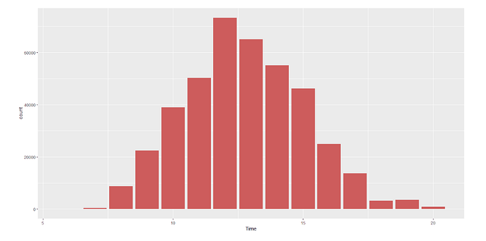
Time of people purchasing items

- This figure answers the question at what time do people often purchase online.
- There has been a clear difference between the hour of day and order volume.
- Most orders happened between 10:00–15:00.
- This helps the retailers to show more advertisements during this peak hour combined with the similar products from Market Basket Analysis.
Number of items each customer buy

- The figure represents how many items each customer bought. People mostly purchased less than 10 items (less than 10 items in each invoice).
The top 20 best selling items

- The figure above represents the top twenty list of bestsellers.
Absolute Item Frequency Plot for top 20 items

- The
absolute item frequency plot()shows the absolute quantity of a certain item that is bought in numbers. - It plots the numeric frequencies of each item independently.
- The
RColorBrewerlibrary adds the colour to the plot.
Relative Item Frequency Plot for top 20 items

- The
relative item frequency plot()shows the relative quantity of a certain item that is bought in percentage. - This graph here shows the
relative item frequencyof top 20 items and the most frequently bought item isWHITE HANGING HEART T-LIGHT HOLDER. - The
RColorBrewerlibrary adds the colour to the plot.
Scatter Plot for the given data (49122 rules)

- The
scatter plot()is a plot for visualising the association rules where the darkness demonstrates thelift, the x axis is thesupportand the y axis is theconfidence. - This is a plot for the 49122
rulesextracted from the Dataset 1. - This demonstrates that most of the items have a
supportof less than 0.002. - It also shows that lift is maximum when the
supportis less. - The
confidencelevel in Dataset 1 is much higher than in Dataset 2 (shown later). Thescatterplotin Dataset 1 are all clustered around 0.01, but for Dataset 1, a neat trend is observed — logistically moving towards Dataset 2 assupportincreases. - As the rules in the Dataset 1 are much higher than in the Dataset 2, it depicts the real world analysis in a better way and hence provides a better scatter plot.
- This concludes the observation with an amazing result that as the number of extracted
rulesincreases, theconfidencelevel tends to one, giving us an accurate result.
A Two Key Plot for the given data (49122 rules)

- The
Two-key plot()is like thescatter plotshowing the x axis assupport, y axis asconfidenceand the colour changes as per theliftas shown in the right. - This graph here shows the
two-key plotfor the whole 49122rulesextracted from the database 1. - It also shows that
liftis maximum when thesupportis less.
Parallel Coordinates Plot for the rules

- The
Parallel Coordinates Plot()shows what products with what items produce what kind of sales. - This is a
parallel coordinates plotfor 50rulesfrom the database. - It shows that if someone buys
BILLBOARD FONTS DESIGN, they buyWRAPnext and the darker colour shows that theconfidenceis high.
Dataset 2
This dataset from Department of Statistics and Biostatistics, California State University can be broken in different ways to make a lot of different inferences.
Relative Item Frequency for the Top 10 Items

- The
itemFrequencyPlot()allows us to show the absolute or relative values. - The figure above shows the
relative item frequencyfor the top 10 items in the first dataset. - It plots how many times these items have appeared as compared to others.
Whole milkis the best selling product, followed byrolls/bunsand othervegetables.
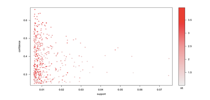
Scatter Plot for the given data (463 Rules)

- The
scatter plot()is a plot for visualising the association rules where the darkness demonstrates thelift, the x axis is thesupportand the y axis is theconfidence. - This is a plot for the 463
rulesextracted from the Dataset 2. - This demonstrates that most of the items have a
supportof less than 0.03. - It also shows that
liftis maximum when thesupportis less.
Graph for top 50 Rules for Association Rules

- The
graph rules plot()is a plot where we can visualise the associationruleseasily. - The size of the bubble increases with the
supportwhile the colour darkens as theliftincreases. - The arrows here indicate what items are bought next to the previous item.
- In this plot,
sausageis bought aftersliced cheese. - The range of
supportandliftis also given in the top right corner.
Parallel coordinates plot for 100 Rules

- The
Parallel Coordinates Plot()shows what products with what items produce what kind of sales. - This is a
parallel coordinates plotfor 100rulesfrom the database. - It shows that if someone buys
berries, they are more likely to buywhipped/sour creamnext and the darker colour shows that theconfidenceis high.
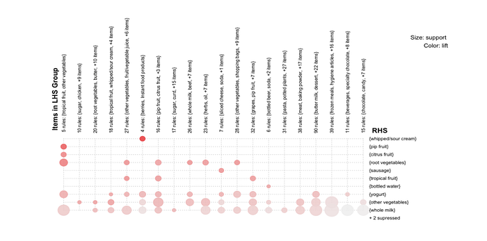
Grouped Matrix for 463 Rules

- In this figure of
grouped matrix plot(), therulesare represented as a grouped matrix-based visualisation. - It is a novel way of creating nested groups of
rules(more specifically antecedent itemsets) via clustering. - The creation of the nested groups form a hierarchy which will be interactively explored to each individual rule.
- The
supportandliftmeasures are represented by the size and color of the balloons, respectively. - In this case it’s not a very useful visualization, since we only have
whipped/sour creamon the right-hand-side of the rules.
Final Words
Market basket analysis is an unsupervised machine learning technique that can be useful for finding patterns in transactional data. It can be a very powerful tool for analyzing the purchasing patterns of consumers.
The main algorithm used for market basket analysis is the apriori algorithm. The three statistical measures in market basket analysis are support, confidence, and lift.
Market basket analysis with the help of association rules can easily tell the customer buying behavior; and the retailer with the help of these concepts can easily setup his retail shop accordingly to expand the business in future.
Although Market Basket Analysis conjures up pictures of shopping carts and supermarket shoppers, it is important that it can be applied to:
- Analysis of credit card purchases
- Analysis of telephone calling patterns
- Identification of fraudulent medical insurance claims
(Consider cases where common rules are broken) - Analysis of telecom service purchases
In this article, we examined the transactional patterns of grocery purchases and discovered both obvious and not-so-obvious patterns in certain transactions.
Finally, If you faced any difficulties, feel free to contact me for any doubts.


